Computing SHAP values from scratch
Recently I tested shap feature importances. SHAP is a novel way of computing which features contributed the most towards the prediction. Whereas the method itself can be generalised to any classifier, it is especially well-suited for tree-based models.
In this blog post I will try to explain what SHAP values are and why I find them very compelling. Following Feynman’s “what I cannot create, I do not understand”, let’s try to compute SHAP feature contributions via a simple example.
import pandas as pd
import matplotlib.pyplot as plt
from sklearn.datasets import load_boston
from sklearn.tree import DecisionTreeRegressor, plot_tree
d = load_boston()
df = pd.DataFrame(d['data'], columns=d['feature_names'])
y = pd.Series(d['target'])
df = df[['RM', 'LSTAT', 'DIS', 'NOX']]
clf = DecisionTreeRegressor(max_depth=3)
clf.fit(df, y)
fig = plt.figure(figsize=(20, 5))
ax = fig.add_subplot(111)
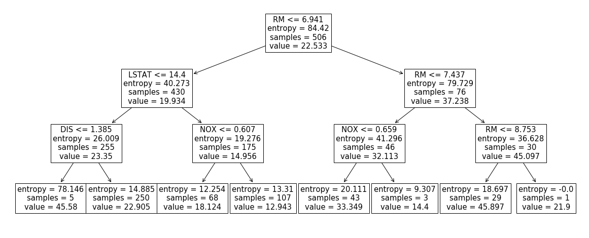
_ = plot_tree(clf, ax=ax, feature_names=df.columns)Above I grabbed a Boston dataset, restricted it to 4 columns ['RM', 'LSTAT',
'DIS', 'NOX'] and built a decision tree, depicted below.
First, let’s compute the shap values for the first row using the official implementation:
import shap
import tabulate
explainer = shap.TreeExplainer(clf)
shap_values = explainer.shap_values(df[:1])
print(tabulate.tabulate(pd.DataFrame(
    {'shap_value': shap_values.squeeze(),
     'feature_value': df[:1].values.squeeze()}, index=df.columns),
tablefmt="github", headers="keys"))| shap_value | feature_value | |
|---|---|---|
| RM | -2.3953 | 6.575 |
| LSTAT | 2.46131 | 4.98 |
| DIS | -0.329802 | 4.09 |
| NOX | 0.636187 | 0.538 |
Note: one nice property of SHAP contributions is that their sum + sample mean is the same as the prediction:
> shap_values.sum() + clf.tree_.value[0].squeeze()
22.905199364899673
> clf.predict(df[:1])
array([22.9052])
Below we’ll figure out why that’s the case. For now, let’s start on computing those values “by hand”.
Shapley values
The underlying computation behind shap feature contributions is powered by a
solution taken from game theory. The setup in our case is as follows:
\(N=4\) features are now allowed to form coalitions. The worth, \(v\), of a
coalition ['RM', 'LSTAT'] is simply
i.e. the prediction of the classifier if only values of RM and LSTAT are
known. Following
solution from the wikipedia page we can now redistribute total “winnings”, \(v(RM, LSTAT, DIS, NOX) - v()\), fairly so that each feature \(i\) gets \( \varphi_{i} \) contribution. Remark that total “winnings” is simply \(E[y|LSTAT=4.98,NOX=0.538,DIS=4.09,RM=6.575] - E[y]\)
where
E[y]=np.mean(y)=clf.tree_.value[0].squeeze()=22.5328and
E[y|LSTAT=4.98,NOX=0.538,DIS=4.09,RM=6.575]=clf.predict(df[:1])=22.9052In English, we want to attribute how much we deviate from the naive prediction
(sample mean) to each feature. Expanding the formula above we get that feature
contribution of RM, \( 4 \varphi_{i} \), is
E[y|RM=6.575] - E[y] +
(E[y|LSTAT=4.98,RM=6.575] - E[y|LSTAT=4.98])/3 +
(E[y|NOX=0.538,RM=6.575] - E[y|NOX=0.538])/3 +
(E[y|DIS=4.09,RM=6.575] - E[y|DIS=4.09])/3 +
(E[y|LSTAT=4.98,NOX=0.538,RM=6.575] - E[y|LSTAT=4.98,NOX=0.538])/3 +
(E[y|LSTAT=4.98,DIS=4.09,RM=6.575] - E[y|LSTAT=4.98,DIS=4.09])/3 +
(E[y|NOX=0.538,DIS=4.09,RM=6.575] - E[y|NOX=0.538,DIS=4.09])/3 +
E[y|LSTAT=4.98,NOX=0.538,DIS=4.09,RM=6.575] - E[y|LSTAT=4.98,NOX=0.538,DIS=4.09]
For the sake of brevity, I would like to omit the explanation of the intuition behind such formula. However I found skim-reading this article and watching this video helping me with understanding why Shapley values are calculated this way.
Figuring out conditional expectations
The remaining question is now how can we compute the conditional expectations in the above formula. Remember I said that SHAP method can in principle be applied to any classifier? The reason behind this is that
E[y|LSTAT=4.98,NOX=0.538,RM=6.575]is just a prediction if DIS value for the feature was not known. We could, in
theory, retrain without the DIS feature and get a classifier to output this
quantity. Or, alternatively, we could marginalise by ranging over observed
DIS values, getting a prediction, and taking a weighted sum according to how common
the value of DIS is. However, all of those methods are prohibitively slow.
In the past I tried to approximate this quantity with the mode of DIS
distribution: however it only worked in a binary classification case.
Turns out in a tree-based classifier, such quantity is easy to compute. Look at our tree again:
Our row forces us to walk the leftmost path of the tree. However, once we hit
the DIS <= 1.385 node we’re not sure where to go as DIS is unknown.
Solution: go both left and right and take a weighted sum. In other words:
E[y|LSTAT=4.98,NOX=0.538,RM=6.575] = 5/255 * 45.58 + 250/255 * 22.905 = 23.3496Let’s write some code that does this for us:
def pred_tree(clf, coalition, row, node=0):
    left_node = clf.tree_.children_left[node]
    right_node = clf.tree_.children_right[node]
    is_leaf = left_node == right_node

    if is_leaf:
        return clf.tree_.value[node].squeeze()

    feature = row.index[clf.tree_.feature[node]]
    if feature in coalition:
        if row.loc[feature] <= clf.tree_.threshold[node]:
            # go left
            return pred_tree(clf, coalition, row, node=left_node)
        # go right
        return pred_tree(clf, coalition, row, node=right_node)

    # take weighted average of left and right
    wl = clf.tree_.n_node_samples[left_node] / clf.tree_.n_node_samples[node]
    wr = clf.tree_.n_node_samples[right_node] / clf.tree_.n_node_samples[node]
    value = wl * pred_tree(clf, coalition, row, node=left_node)
    value += wr * pred_tree(clf, coalition, row, node=right_node)
    return value

> pred_tree(clf, coalition=['LSTAT', 'NOX', 'RM'], row=df[:1].T.squeeze())
23.349803921568633
Putting it all together
from itertools import combinations
import scipy

def make_value_function(clf, row, col):
    def value(c):
        marginal_gain = pred_tree(clf, c + [col], row) - pred_tree(clf, c, row)
        num_coalitions = scipy.special.comb(len(row) - 1, len(c))
        return marginal_gain / num_coalitions
    return value

def make_coalitions(row, col):
    rest = [x for x in row.index if x != col]
    for i in range(len(rest) + 1):
        for x in combinations(rest, i):
            yield list(x)

def compute_shap(clf, row, col):
    v = make_value_function(clf, row, col)
    return sum([v(coal) / len(row) for coal in make_coalitions(row, col)])

print(tabulate.tabulate(pd.DataFrame(
    {'shap_value': shap_values.squeeze(),
     'my_shap': [compute_shap(clf, df[:1].T.squeeze(), x) for x in df.columns],
     'feature_value': df[:1].values.squeeze()
    }, index=df.columns),
tablefmt="github", headers="keys"))| shap_value | my_shap | feature_value | |
|---|---|---|---|
| RM | -2.3953 | -2.3953 | 6.575 |
| LSTAT | 2.46131 | 2.46131 | 4.98 |
| DIS | -0.329802 | -0.329802 | 4.09 |
| NOX | 0.636187 | 0.636187 | 0.538 |
And there you have it: we have replicated the computations in the shap
library. When SHAP values are computed for a forest of decision trees, we
simply average those. Because SHAP contributions are Shapley values we get
certain desired properties “for free”:
- contributions + bias = prediction
- contributions of irrelevant features are 0
- consistency: changing a model so a feature has a larger impact on the model will never decrease the contribution assigned to that feature
and thus I have become an advocate for using this method.
Final thoughts
In my eyes, the genius of Scott M. Lundberg, Gabriel G. Erion, and Su-In Lee
who published the shap library isn’t that they used Shapley values: this has
been known prior to them by Strumbelj, Erik, and Igor Kononenko all the way
back in 2014, but the fact that they invented a fast pred_tree algorithm. The
primitive recursive algorithm presented in this blog post would be too slow to
deploy in a live system for any reasonably-sized tree. When faced with a similar
problem of computing conditional expectations in the past and I ended up
approximating these by going down the path that is closest to the current value
instead of taking the weighted average of the children. My hacky solution makes
computations of contributions just as fast as predictions however it is less
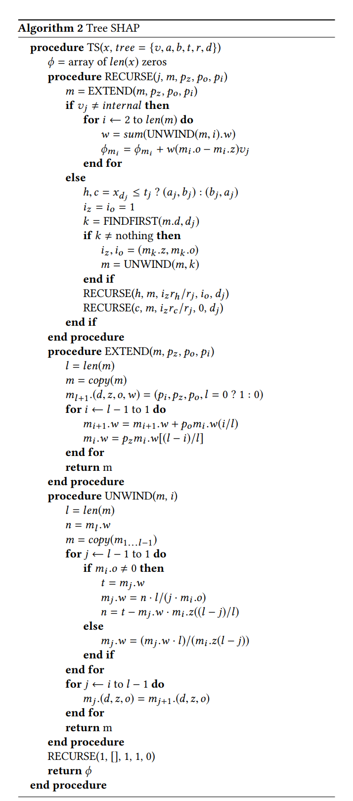
robust. I include the fast “Algorithm 2” from the tree shap paper, but, after
staring at it for a few days by now, I have given up on any hope of
understanding it just by reading it. Perhaps some motivated reader could email
me the explanation. For now, this is good bye!