Motivation
- A policeman spots an armed person next to a robbery. He quickly concludes that the man is guilty. By what reasoning process?

Artiom Fiodorov (Tom)
October, 2015
The reasoning of our policeman consists of the following weak syllogisms:
Strong syllogisms can be chained together without any loss of certainty
Weak syllogism have wider applicability
Most of the reasoning people do consists of weak syllogism.
Answer: yes, using probability theory.
A state of information \(X\) summarises the information we have about some set of atomic propositions \(A\), called the basis of \(X\), and their relationships to each other. The domain of \(X\) is the logical closure of \(A\).
\(A, X\) is the state of information obtained from \(X\) by adding the additional information that \(A\) is true.
(R1) (A | X) is a single real number. There exists a single real number \(T\) such that \((A | X) \leq T\) for every \(X\) and \(A\).
\(X\) is consistent if there's no proposition \(A\) such that \((A | X) = T\) and \((\neg A | X) = T\).
(R2) Plausibility assignment are compatible with propositional calculus
(R3) There exists a non increasing function \(S_0\) such that \((\neg A | X) = S_0 ( A | X)\) for all \(A\) and consistent X.
Proposition: \(F := S_0(T)\). Then \(F \leq (A | X) \leq T\) for all \(A\) and consistent X.
(R4) (Universality) There exists a nonempty set of real numbers \(P_0\) with the following two properties
(R5) (Conjunction) There exists a continuous function \(F:[F, T]^2 \to [F, T]\), such that \((A \wedge B | X) = F((A | B, X), (B | X))\) for any \(A, B\) and consistent \(X\).
Heuristic: for \(A \wedge B\) to be true \(B\) has to be true so \((B | X)\) is needed. If \(B\) is false then \(A \wedge B\) is false independently of \(A\), so \((A | X)\) is not needed if \((A | B, X)\) and \((B | X)\) are known.
There exists a continuous, strictly increasing function \(p\) such that, for every \(A, B\) consistent with \(X\),
Kolmogorov's probability is defined on a sample space \(\Omega\) with an event space \(F\) which forms a \(\sigma\)-algebra
Example: Coin toss. Then \(\Omega = \{H, T\}\), \(F = \{ \emptyset, \{H\}, \{T\}, \{H, T\} \}\). Sample measure \(P\) is then just \(P(\{H\}) = P(\{T\}) = 1/2\), \(P(\emptyset) = 0\), \(P(\{H, T\}) = 1\).
To relate frequencies with plausibilities we will use MaxEnt principle
\(1/6\) to each outcome is ruled out as the average would be \(3.5\).
Solution: out of all probability distributions that average to \(4\) pick the one which maximise the information entropy: \(\sum_{j = 1}^{6} -p_j \log p_j\).
Start with \(n\) independent trials, each with different \(m\) outcomes.
Each sample is then just a string of length \(n\):
\[ 1, m-1, m-2, 5, 6, 7, 3, 1, 2, 3, 5, 7\]
So sample space is \(S^n = \{1, 2, \dots, m\}^n\) such that \(|S^n| = m^n\).
Start with "ignorance knowledge" \(I_0\) i.e.
\[ P(A | I_0) = \frac{M(n, A)}{|S^n|} \,,\]
where the multiplicity of \(A\), \(M(n, A)\), is just the number of distinct strings in \(S^n\) such that \(A\) is true.
Denote by \(n_1, n_2, \dots n_m\) the number of times the trial came up with result \(1, 2, \dots, m\) respectfully.
If the string is \(1, 2, 1, 2, 2, 2, 3\), then \((n_1, n_2, n_3) = (2, 4, 1)\).
Suppose we have a restriction \(R\) where \(A(n_1, n_2, \dots, n_m)\) is true. If \(A\) is linear in \(n_j\) then
\[ M(n, A) = \sum_{n_j \in R} \frac{n!}{n_1!n_2!\dots n_m!} \]
Rolling a die \(20\) times. \(A = \text{average roll is 4}\). Then pick \((n_1, n_2, n_3, n_4, n_5, n_6)\) so that \(\sum n_i = 20\). If \(\sum i * n_i = 4 * 20 = 80\), include the multinomial coefficient in the calculation of multiplicity of \(A\):
\begin{align*} M(20, A) = \frac{20!}{1!1!1!12!4!1!} + \frac{20!}{1!1!1!13!2!2!} + \frac{20!}{1!1!2!10!5!1!} + \cdots \end{align*}There are \(283\) terms in the summation.
Let \(W_{\max} = \max_{R} \frac{n!}{n_1! n_2! \dots n_m!}\). Then
\[ W_{\max} \leq M(n, A) \leq W_{\max} * \frac{(n + m - 1)!}{n! (m - 1)!} \]
Can be seen that \(\text{\# of terms} \sim n^{m-1} / (n-1)!\), so
\[ \frac{1}{n} \log M(n, A) \to \frac{1}{n} \log (W_{\max}) \text{ as } n \to \infty\]
Introduce frequency distribution \(f_j = n_j / n\). If \(f_j\)'s tend to constants as \(n \to \infty\), use Stirling's approximation
\[ \frac{1}{n} \log M(n, A) \to H := - \sum_{j = 1}^{m} f_j \log f_j \,.\]
So the multiplicity can be found by determining the frequency distribution \(\{ f_j \}\) which maximises entropy subject to \(R\).
We can further show that for \(A = \sum_{i=1}^{m} g_i n_i\),
\[ P(\text{trial}_i = j | A, n, I_0) = \frac{M(n - 1, A - g_j)}{M(n, G)} = f_j \,. \]
(Trick) set \(g_1 = \pi, g_2 = e\). If \(A(n_2, n_2) = 3 \pi + 5 e\) is true, then \((n_1, n_2) = (3, 5)\). Can be shown that
\[ P(\text{trial}_i = j | \{n_j\}, n, I_0) = \frac{n_j}{n} \]
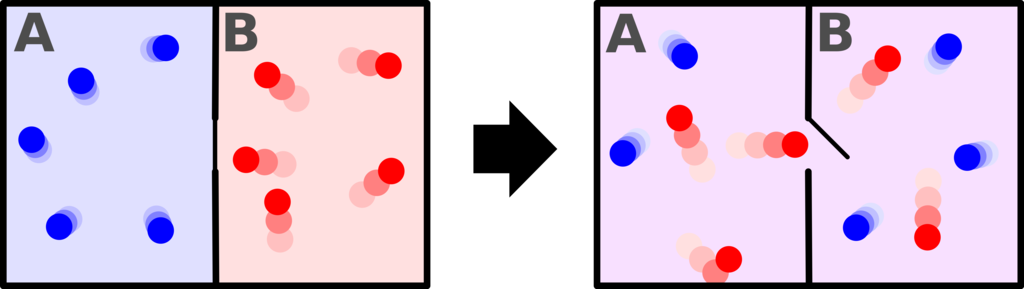
disorder increases
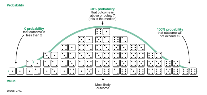
CLT
Let \(X_1, X_2, \dots, X_n\) be independent, identically distributed random variables. Then
\[ \frac{X_1 + X_2 + \dots + X_n - n \mu}{\sqrt{n}} \to \mathcal{N}(0, 1)\]
Why convergence? Why Gaussian?
Turns out: convolution: \(X + Y\) is "forgetful", but keeps mean and variance fixed. And Gaussian is the MaxEnt-distribution with prescribed mean and variance.
Ask everyone in China about the height of the Emperor.
What assumption of the CLT is broken?
Logical independence: \(P(A|BC) = P(A|C)\), so knowledge that \(B\) is true does not affect the probability we assign to A.
Causal independence: no physical cause.
Note: neither imply the other.
"Information theory must precede probability theory and not be based on it." -- Kolmogorov
There are 2 worlds:
Then observing a black crow is evidence against the hypothesis that all crows are black.
Same data can be evidence against and for same hypothesis.
Many of our applications lie outside the scope of conventional probability theory as currently taught. But we think that the results will speak for themselves, and that something like the theory expounded here will become the conventional probability theory of the future.
-- E.T. Jaynes. Probability: The Logic of Science
A scientist who has learned how to use probability theory directly as extended logic has a great advantage in power and versatility over one who has learned only a collection of unrelated ad hoc devices. As the complexity of our problems increases, so does this relative advantage. Therefore we think that, in the future, workers in all the quantitative sciences will be obliged, as a matter of practical necessity, to use probability theory in the manner expounded here.
-- E.T. Jaynes. Probability: The Logic of Science