Getting a musical note from audio
Lately I have been learning music playing around with computers & maths
under the pretence of learning music. I am particularly interested in breaking
down melodies into individual notes. However since actually training my
musical ear is hard work, I am going to use basic signal processing in order to
achieve my goal.
Can you identify the note? Well I can’t. So I am going to use a computer to do this for me.
First, I am going to discover some basics of digital music audio by loading the above audio file & plotting it. I get something like this:
CODE
import librosa
import pandas as pd
import plotly.express as px

note_filepath = "/home/tom/afiodorov.github.io/assets/note.wav"
y, sample_rate = librosa.load(note_filepath, sr=None)
df = pd.DataFrame({'time (s)': np.arange(len(y)) / sample_rate, 'wave': y})
fig = px.line(df, x="time (s)", y="wave", title='Raw Waveform')
fig.show()
Turns out digital audio is represented by a series of real numbers, i.e. it is a one-dimensional array. When we plot our series, we get extremely wiggly line. Such plot is referred to as (raw) waveform. If you zoom in enough in the above chart, you will see that it’s just a line. I found it surprising how easy it is to represent music. The greatest, most complex compositions you have ever listened to are just a bunch of real numbers. Let’s print first 10 numbers of the above file just for illustrative purpose:
y[:10]
> array([-0.03649902, -0.04107666, -0.05935669, -0.09130859, -0.1232605 ,
>        -0.13696289, -0.15524292, -0.17349243, -0.18261719, -0.20089722],
>              dtype=float32)]
Do these 10 numbers sound like a note to you :)? Just kidding. Even if you discovered a way to enjoy music by reading a long list of numbers, these 10 would actually be inaudible: they represent a miniscule part of the 1 second interval above. In the plot above 44 100 points are used to represent 1 second worth of audio. This is the same as saying that the sampling rate of our recording is 44 100 Hz. To put it in elementary terms, we record the audio wave value 44 100 times per second at equally spaced intervals. Why 44 100? This number is linked to human hearing. People can hear sounds from 20 to 20 000 Hz, where the higher the number of Hz, the higher the sound sounds to you. It turns out in order to record audio in such range, we need to sample twice as often, thus the sampling rate of 44 1001 has been used often in digital records.
Basic musical theory: we have 7 notes: do, re, mi, fa, sol, la, si, do, alternatively known as C, D, E, F, G, A, B, C. The latter do is an octave above the first do. What’s an octave from a physical point of view? Turns out if a note has frequency twice as high as another note than those two notes are the same but one octave apart. Often subscript is used to denote octaves, e.g. C₂ and C₃ are one octave apart whereas F₄ and F₇ are 3 octaves apart. At some point in the 20th century musicians all around the world agreed that A₄ (la) is 440 Hz. Now let’s look at notes on a piano:
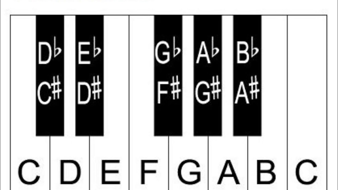
There are actually 12 keys between the two C’s when we count the black keys. These 12 keys are equally separated musically. Curiously there’s no black key between mi (E) & fa (F). The distance between F and G is a tone and the distance between E & F is a semitone. What do I mean by equally separated? The ratio of frequencies matter when we compare notes, as opposed to their absolute frequency. Thus for adjacent notes to have the same ratio I can apply a factor of \( \sqrt[12]{2} \approx 1.06 \) every time I go up by a semitone. This way after I apply it 12 times, I double the frequency and thus complete the octave. Using this knowledge it’s a trivial exercise in computer science to generate frequencies of all notes. I presented to you a cropped table of some of them from octave 0 to 6:
| octave | F# | G | G# | A | A# | B |
|---|---|---|---|---|---|---|
| 0 | 23.1247 | 24.4997 | 25.9565 | 27.5 | 29.1352 | 30.8677 |
| 1 | 46.2493 | 48.9994 | 51.9131 | 55 | 58.2705 | 61.7354 |
| 2 | 92.4986 | 97.9989 | 103.826 | 110 | 116.541 | 123.471 |
| 3 | 184.997 | 195.998 | 207.652 | 220 | 233.082 | 246.942 |
| 4 | 369.994 | 391.995 | 415.305 | 440 | 466.164 | 493.883 |
| 5 | 739.989 | 783.991 | 830.609 | 880 | 932.328 | 987.767 |
| 6 | 1479.98 | 1567.98 | 1661.22 | 1760 | 1864.66 | 1975.53 |
rest of the notes
| octave | C | C# | D | D# | E | F |
|---|---|---|---|---|---|---|
| 0 | 16.3516 | 17.3239 | 18.354 | 19.4454 | 20.6017 | 21.8268 |
| 1 | 32.7032 | 34.6478 | 36.7081 | 38.8909 | 41.2034 | 43.6535 |
| 2 | 65.4064 | 69.2957 | 73.4162 | 77.7817 | 82.4069 | 87.3071 |
| 3 | 130.813 | 138.591 | 146.832 | 155.563 | 164.814 | 174.614 |
| 4 | 261.626 | 277.183 | 293.665 | 311.127 | 329.628 | 349.228 |
| 5 | 523.251 | 554.365 | 587.33 | 622.254 | 659.255 | 698.456 |
| 6 | 1046.5 | 1108.73 | 1174.66 | 1244.51 | 1318.51 | 1396.91 |
CODE
def num_semitones_between(note1: str, note2: str) -> int:
    notes = ['C', 'C#', 'D', 'D#', 'E', 'F', 'F#', 'G', 'G#', 'A', 'A#', 'B']
    return notes.index(note1) - notes.index(note2)

def note_frequency(note: str, octave: int = 4) -> float:
    a_4 = 440 #  standard pitch
    a_frequency = a_4 * 2 ** (octave - 4)
    adjustment = num_semitones_between(note, "A")
    return a_frequency * 2 ** (adjustment / 12)

def gen_notes_table() -> pd.DataFrame:
    l = []
    notes = ['C', 'C#', 'D', 'D#', 'E', 'F', 'F#', 'G', 'G#', 'A', 'A#', 'B']
    for octave in range(7):
        l.append([note_frequency(note, octave=octave) for note in notes])
    df = pd.DataFrame(l, columns=notes)
    df.index.name = 'octave'
    return df

import tabulate
tabulate.tabulate(gen_notes_table(), tablefmt="github", headers="keys")
Note: in the above table the ratio between A# and A is roughly 1.06 (466 / 440), just like advertised.
OK, but how do we get the goddamn note from the audio snippet? We need some sort of transformation of the waveform into frequencies. Fourier transform, an interesting piece of mathematics discovered by Joseph Fourier in 1822, allows us to “pluck out” specific frequencies from the sound and see how much each of them contribute. Graphically it means that we are going to take the waveform shown above, and try to approximate it by adding functions cosine and sine until the result looks almost exactly like our waveform. A process illustrated below for a simple waveform that is of quadratic shape:

The more cosine & sine functions we add, the more precise the approximation becomes. What we are interested in is which exactly cosine & sine contribute the most to the recorded waveform, i.e. which notes are present in the audio? Let’s perform the transform and plot it:
CODE
import numpy as np

ft = np.fft.rfft(y)
df = pd.DataFrame(np.absolute(ft[1:]), index=range(1, len(ft)))
df.index.name = "Frequency (Hz)"
df.columns = ['Amplitude']
df = df.reset_index()
fig = px.line(df[:2000], x="Frequency (Hz)", y="Amplitude", title='Fourier transform')
fig.show()
From the above graph we see that the frequency that is the most present is 370 Hz, meaning the note recorded is F#₄ (fi). Interestingly enough F#₅ (740 Hz) and F#₆ (≈ 1486 Hz) are also present. These are so-called overtones that make the sound sound more pleasant. Whew, so much maths to identify the note, but we finally got here! Finally, I am including two more audio samples, for educational purposes.
-
Why 44 100 as opposed to 40 000? I don’t know! ↩